NBPhO 2025

Part i (3 points)

Both aluminium plates were immersed in hot water until thermal equilibrium was reached, then removed, dried with tissue paper, and measured using an infrared thermometer. The plates have identical thermal properties except for their surface coating, so they should have reached the same actual temperature in the hot water bath. Experimental measurements:

$T_\text{polished}$ (°C)	$T_\text{black}$ (°C)	$T_\text{room}$ (°C)
26.2	70.9	22.9
26.0	70.7	22.9
25.4	70.2	22.9

The infrared thermometer measures temperature based on thermal radiation and is calibrated for emissivity $\varepsilon = 1$ (in reality $\varepsilon = 0.95$, but this difference is not significant). The radiation power can be linearized: $P_\text{thermal} = P_0 + \alpha T$. Objects with $\varepsilon < 1$ radiate $P_\varepsilon = \varepsilon(P_0 + \alpha T_\varepsilon)$, but they also reflect/scatter the radiation from the environment. If the room is at thermal equilibrium at temperature $T_0$, the room is filled with photons at equilibrium with walls at temperature $T_0$. As it follows from the second law of thermodynamics, the reflectance must be $1 - \varepsilon$, so it reflects/scatters power equal to $P_r = (1-\varepsilon)(P_0 + \alpha T_0)$. The total power departing from it is $P_\varepsilon + P_r = P_0 + \varepsilon\alpha T_\varepsilon + (1-\varepsilon)T_0$. The IR thermometer equates this to $P_0 + \alpha T_\text{reading}$, hence the reading is a weighted average:

$$T_\text{reading} = \varepsilon\cdot T_\varepsilon + (1-\varepsilon)\cdot T_0.$$

Since the black plate has $\varepsilon = 1$, its reading directly gives the actual temperature of both plates. Rearranging to solve for emissivity:

$$\varepsilon = \frac{T_\text{polished} - T_0}{T_\text{black} - T_0}.$$

Calculating for each measurement:

$$\varepsilon_1 = \frac{26.2 - 22.9}{70.9 - 22.9} = 0.069, \quad \varepsilon_2 = \frac{26.0 - 22.9}{70.7 - 22.9} = 0.065, \quad \varepsilon_3 = \frac{25.4 - 22.9}{70.2 - 22.9} = 0.053.$$

Taking the average: $\varepsilon = (0.069 + 0.065 + 0.053)/3 = 0.062 \approx 0.06$.

The emissivity of the polished aluminium plate is $\varepsilon = 0.06 \pm 0.01$.

Grading (preliminary)

• The idea of heating the two plates together in water: 0.4 pts
• Measuring the radiance of the plates properly (plates are properly dried and measurements are done in a timely manner): 0.4 pts
• Making at least three measurements of the black plate, the polished plate and the surrounding environment (0.2 pts for each set of 3, totalling): 0.6 pts
• Understanding that the IR temperature reading of the polished plate is affected not only by the plate itself, but also by the reflected radiation of the environment ($T_\text{reading} = \varepsilon\cdot T_\text{actual} + (1-\varepsilon)\cdot T_\text{ambient}$, not just $T_\text{reading} = \varepsilon\cdot T_\text{actual}$): 0.3 pts
• Deriving a correct formula for emissivity, expressed in terms of the three measured temperatures: 0.7 pts
• Calculated value of emissivity in the range from 0.03 to 0.12: 0.6 pts (for values from 0.02 to 0.2: 0.4 pts; for values from 0.01 to 0.3: 0.2 pts)

---

Part ii (3 points)

Solution 1. Here the main idea is to heat the plate using the resistor. Once thermal equilibrium is reached with the plate’s temperature $T = T_f$, the heating power $P = V^2/R$ equals the power dissipated to the environment, $H(T_f - T_0)$ (with $T_0$ denoting the room temperature), hence

$$H = \frac{V^2/R}{T_f - T_0}.$$

The main difficulty is that the characteristic thermalization time is long (around 7 minutes), so for a more or less precise measurement, one should wait around half an hour.

Solution 2. The black aluminium plate was placed on the foam plastic with the resistor beneath it, providing continuous heating. Temperature readings were recorded at one-minute intervals:

$t$ (min)	0	1	2	3	4	5	6
$T$ (°C)	28.0	30.8	33.2	35.2	37.3	39.0	40.3

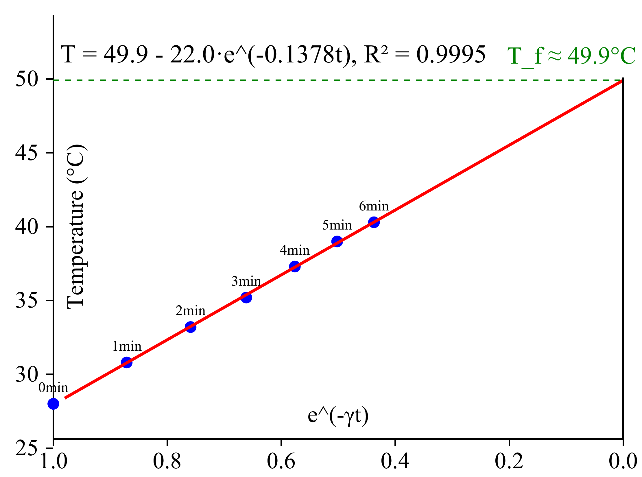
For heating with constant power, the temperature evolution follows $T = T_f - \theta e^{-\gamma t}$, where $T_f$ is the final equilibrium temperature, $\theta$ is a constant depending on the initial temperature, and $\gamma$ is the inverse of the characteristic time constant. To determine $\gamma$, we examine successive temperature increments $T(t+\tau) - T(t) = \theta e^{-\gamma t}(e^{\gamma\tau} - 1)$ with $\tau = 1\,\text{min}$, which should decrease exponentially:

$$\ln\Delta T \equiv \ln[T(t+\tau) - T(t)] = -\gamma t + \text{const}.$$

$t$ (min)	$\Delta T$ (°C)	$\ln(\Delta T)$
0	2.80	1.0296
1	2.40	0.8755
2	2.00	0.6931
3	2.10	0.7419
4	1.70	0.5306
5	1.30	0.2624

Linear regression of $\ln[T(t+1) - T(t)]$ versus $t$ yields $\ln[T(t+\tau) - T(t)] = 1.0333 - 0.1378t$ with $R^2 = 0.9209$, giving $\gamma = 0.1378\,\text{min}^{-1}$ (time constant $1/\gamma \approx 7.3\,\text{min}$).

We then plot $T$ versus $e^{-\gamma t}$ to find $T_f$ as the intercept when $e^{-\gamma t} = 0$. Linear regression yields $T_f \approx 49.9\,°\text{C}$:

$$T = 49.9 - 22.0\cdot e^{-0.1378t}, \quad R^2 = 0.9995.$$

At thermal equilibrium the power dissipated equals the power supplied:

$$P = \frac{U^2}{R} = h\cdot A\cdot(T_f - T_0) = H\cdot(T_f - T_0).$$

Using $U = 15\,\text{V}$, $R = 220\,\Omega$, $A = 40\times 40\,\text{mm}^2 = 1.6\times 10^{-3}\,\text{m}^2$ and $T_0 = 22.9\,°\text{C}$:

$$h = \frac{U^2/R}{A\cdot(T_f - T_0)} \approx 23.6\,\text{W\,m}^{-2}\text{K}^{-1}, \quad H = h\cdot A = 37.8\,\text{mW\,K}^{-1}.$$

Grading for Solution 1 (preliminary)

• The idea of using resistive heating and waiting for thermalization: 0.5 pts
• For waiting long enough, up to 0.8 pts: for each five minutes missing from more than 30 minutes, subtract 0.2 pts
• The voltage is maximized to have maximal $T_f$ (needed to reduce the relative error of $T_f - T_0$): 0.4 pts (the maximal allowed voltage of 15 V gives maximal points; each missing volt subtracts 0.1 pts)
• Measuring the temperature and obtaining a value that is reasonable for the given voltage (difference not bigger than 1 °C): 0.6 pts
• Deriving a correct formula for $H$: 0.5 pts
• Evaluating correctly: 0.2 pts (any mistake, either with units or arithmetic, leads to no points)

Grading for Solution 2 (preliminary)

• Coming up with the idea of analysing exponential decay of temperature change with a graph and deriving the heat transfer coefficient from that: 0.5 pts
• Correct equation $T(t) = T_f - \theta e^{-\gamma t}$: 0.3 pts
• Plotting the data to a graph to determine $\gamma$ and to confirm the validity of collected data: 0.3 pts
• At least 5 datapoints used: 0.1 pts
• Measure for at least 5 minutes: 0.1 pts
• Calculating the slope and retrieving $\gamma$ from it: 0.2 pts
• Finding the maximal temperature for used voltage, using plot of $T$ vs $e^{-\gamma t}$: 0.5 pts
• Evaluating $P = U^2/R = h\cdot A\cdot(T_f - T_0) = H\cdot(T_f - T_0)$ without errors: 0.5 pts
• Getting heat transfer coefficient close to expected value: 0.5 pts

---

Part iii (2 points)

Solution 1. To determine the heat capacity, we use the heating curve from Part ii. During heating, the energy balance is

$$P_\text{in} - P_\text{out} \equiv \Delta P = C\frac{dT}{dt},$$

where $P_\text{in} = U^2/R$, $P_\text{out} = H(T - T_0)$, and $C$ is the heat capacity. Using the exponential model $T = T_f - \theta e^{-\gamma t}$:

$$\frac{dT}{dt} = \theta\gamma e^{-\gamma t} = \gamma(T_f - T).$$

Substituting:

$$P_\text{in} - H(T - T_0) = C\gamma(T_f - T), \quad \text{hence} \quad C = \frac{P_\text{in} - H(T - T_0)}{\gamma(T_f - T)}.$$

Using $U = 15\,\text{V}$, $R = 220\,\Omega$, $H = 3.78\times 10^{-2}\,\text{W\,K}^{-1}$, $T_0 = 22.9\,°\text{C}$, $T_f = 49.9\,°\text{C}$, $\gamma = 0.1378\,\text{min}^{-1}$, the input power is $P_\text{in} = 15^2/220 = 1.023\,\text{W}$.

$t$ (min)	$T$ (°C)	$P_\text{out}$ (W)	$\Delta P$ (W)	$dT/dt$ (K/min)	$C$ (J/K)
0	28.0	0.193	0.830	3.018	16.5
1	30.8	0.299	0.724	2.629	16.5
2	33.2	0.389	0.633	2.291	16.6
3	35.2	0.465	0.558	1.996	16.7
4	37.3	0.544	0.478	1.739	16.5
5	39.0	0.609	0.414	1.515	16.4
6	40.3	0.658	0.365	1.320	16.6

The heat capacity values are remarkably consistent, validating our model. Taking the average yields $C \approx 16.5\,\text{J\,K}^{-1}$.

For reference, $c_\text{Al} = 900\,\text{J\,kg}^{-1}\text{K}^{-1}$, so the plate mass is $C/c_\text{Al} = 18.3\,\text{g}$, consistent with a $40\,\text{mm}\times 40\,\text{mm}$ plate with thickness approximately 2 mm.

Solution 2. A better approach is to make an additional series of measurements to obtain a cooling temperature curve, excluding the contribution of the resistor’s thermal capacity. We heat the plate (easiest by immersing in hot water) and measure $T(t)$ as it cools. The energy balance gives

$$P_\text{out} = H[T(t) - T_0] = -C\frac{dT}{dt} = \gamma C[T(t) - T_0], \quad \text{hence} \quad C = H/\gamma.$$

The decay rate $\gamma$ is found from the slope of $\ln[T(t) - T_0]$ plotted against $t$.

Grading (preliminary)

• The idea of using the $T(t)$ dependence, either for cooling or heating with the resistor: 0.2 pts
• Measuring and tabulating at least 6 data points: 0.3 pts (subtract 0.1 pts for each missing)
• Data points cover at least 6 minutes: 0.3 pts (subtract 0.1 pts for each missing minute)
• The idea of using log-linear plot for data linearization: 0.2 pts
• Correct data plotting: 0.2 pts
• Finding the slope of a fit line: 0.2 pts
• The idea of substituting time derivative with multiplication by $\gamma$: 0.2 pts (calculating derivative by finite difference ratio $\Delta T/\delta t$ is significantly less accurate)
• Deriving a correct formula for $C$: 0.2 pts
• Obtaining a reasonable numerical value for $C$, from 13 to 20 J/K: 0.2 pts (else from 10 to 25 J/K: 0.1 pts)

---

Part iv (4 points)

Cooling experiments were conducted with the aluminium plate covered by different numbers of silicone rubber layers. The plate was heated in water and allowed to cool, with temperature recorded as a function of time.

$t$ (s)	0	60	120	180	240	300
$T_{1\,\text{layer}}$ (°C)	65.2	60.2	55.5	51.3	47.6	44.6
$T_{2\,\text{layers}}$ (°C)	*	35.3	34.0	32.9	31.9	30.8
$T_{3\,\text{layers}}$ (°C)	45.4	43.1	41.6	40.0	38.9	37.3

*The data point at $t = 0$ for 2 layers is excluded as it did not represent complete thermal equilibrium across the silicone layers.

For a cooling process with constant ambient temperature $T_0$, the temperature follows exponential decay $T(t) = T_0 + (T_\text{initial} - T_0)e^{-\gamma t}$. The time constant $\gamma$ is related to the thermal resistance $\mathcal{R}$ and heat capacity $C$ by

$$\gamma = \frac{1}{\mathcal{R}C}.$$

Taking the natural logarithm of the temperature difference from ambient yields $\ln[T(t) - T_0] = -\gamma t + \text{const}$.

Using linear regression on the logarithmic cooling curves:

$$\gamma_{1\,\text{layer}} = 2.244\times 10^{-3}\,\text{s}^{-1}, \quad \gamma_{2\,\text{layers}} = 1.852\times 10^{-3}\,\text{s}^{-1}, \quad \gamma_{3\,\text{layers}} = 1.438\times 10^{-3}\,\text{s}^{-1}.$$

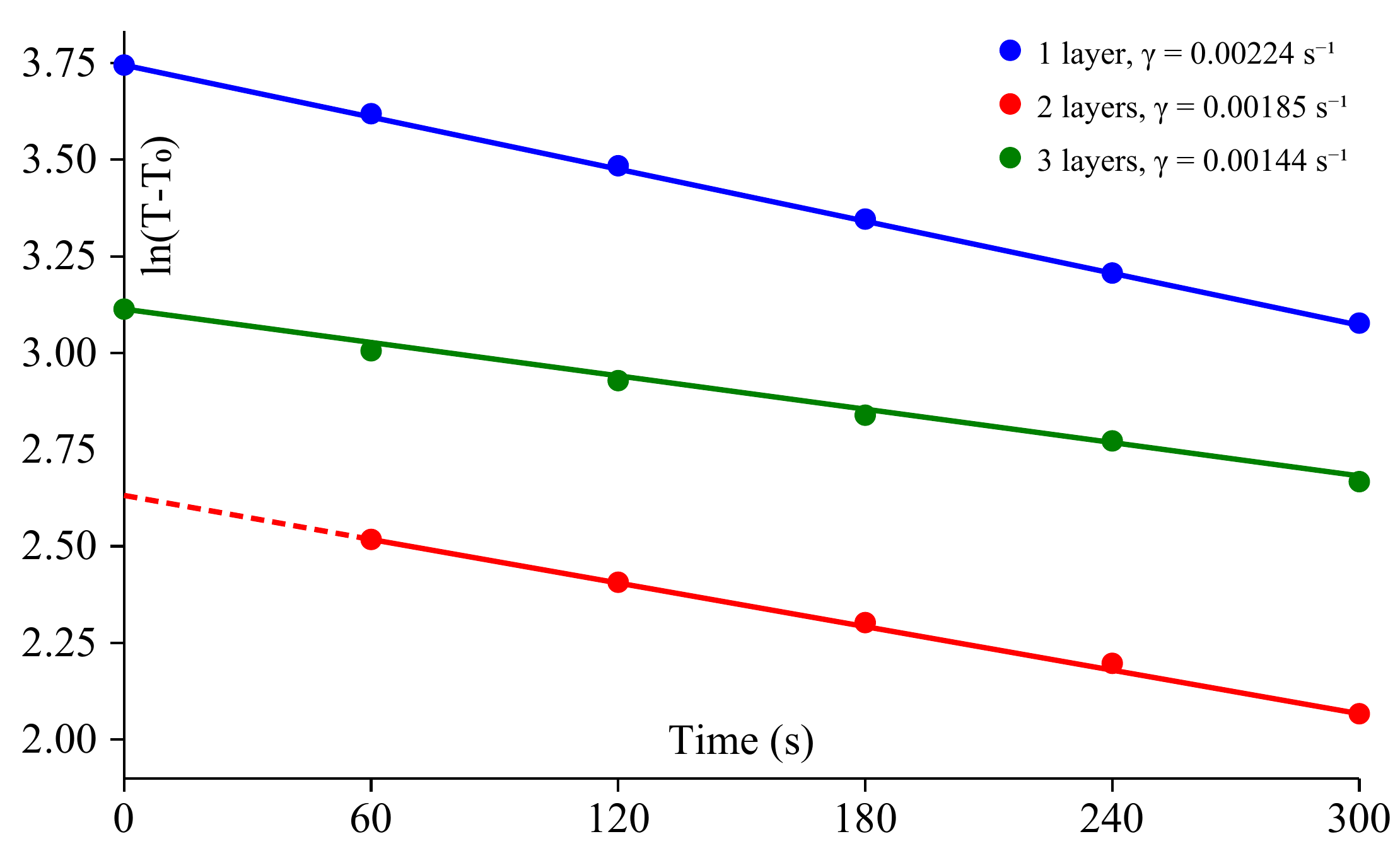
Using $C = 16.5\,\text{J\,K}^{-1}$, the total thermal resistance for each case is:

$$R_{1\,\text{layer}} = \frac{1}{\gamma_{1}\cdot C} = 27.0\,\text{K\,W}^{-1}, \quad R_{2\,\text{layers}} = 32.7\,\text{K\,W}^{-1}, \quad R_{3\,\text{layers}} = 42.1\,\text{K\,W}^{-1}.$$

Each additional layer adds a resistance $\Delta R = \delta/(\kappa A)$, where $\delta$ is the layer thickness, $\kappa$ is the thermal conductivity, and $A$ is the area. The incremental resistances are:

$$\Delta R_{12} = R_{2\,\text{layers}} - R_{1\,\text{layer}} = 5.7\,\text{K\,W}^{-1}, \quad \Delta R_{23} = R_{3\,\text{layers}} - R_{2\,\text{layers}} = 9.4\,\text{K\,W}^{-1}.$$

Taking the average:

$$\overline{\Delta R} = \frac{\Delta R_{12} + \Delta R_{23}}{2} = 7.6\,\text{K\,W}^{-1}.$$

With $\delta = 0.8\,\text{mm} = 8\times 10^{-4}\,\text{m}$ and $A = 40\times 40\,\text{mm}^2 = 1.6\times 10^{-3}\,\text{m}^2$:

$$\kappa = \frac{\delta}{\overline{\Delta R}\cdot A} = 0.066\,\text{W\,m}^{-1}\text{K}^{-1}.$$

Grading (preliminary)

• The idea of letting the plate cool down while covering it with a different number of silicon sheets and measuring the $T(t)$ dependencies: 0.3 pts
• For the quantity of recorded data: within each data series, at least 6 data points: 0.3 pts (subtract 0.1 for each missing); within up to three different data series — in total up to $3\times 0.3 = 0.9$ pts
• Data points in each data series cover at least 6 minutes: 0.2 pts (0.1 pts if less than 6 but more than 4 minutes) — in total up to 0.6 pts
• The idea of using log-linear plot for data linearization: 0.2 pts
• Correctly plotting the data: 0.1 pts each, up to 0.3 pts
• Calculating $\gamma$ for each of the series, 0.1 pts for each, in total up to 0.3 pts
• Correctly expressing the heat conductivity in terms of a difference of the $\gamma$ values: 0.7 pts
• Finding conductivity on the basis of all the $\gamma$ values (either by pair-wise calculation, or plotting and finding the fit line slope): 0.4 pts (divide by two if only one pair of $\gamma$ values was used)
• Obtained value of $\kappa$ within a reasonable range, i.e. from 0.05 to 0.1 W m$^{-1}$ K$^{-1}$: 0.3 pts (else if from 0.04 to 0.12: 0.2 pts; else from 0.02 to 0.14: 0.1 pts)