NBPhO 2025

Part i (1 point)

Gravitational acceleration obeys Gauss’ law, i.e., the number of field lines passing through a closed surface is proportional to the enclosed mass. We can see from the example of a point mass $M$ that $\int g\,dA = 4\pi GM$. Applied for the case of an infinite plane with constant density $\rho_0$ with a cuboid of area $A$ and half-thickness $z$, we get $-2a_z A = 4\pi G\cdot 2Az\rho_0$, so

$$a_z = -4\pi G\rho_0 z.$$

Grading (preliminary)

• Idea of using Gauss’ law: 0.3 pts
• Formula relating the mass inside with gravitational flux: 0.3 pts
• Application of Gauss’ law on a cuboid: 0.2 pts
• Final result: 0.2 pts

Alternative solution:

• Finding the acceleration of a thin disk by integrating over its surface: 0.5 pts
  • Writing down the integral: 0.3 pts
  • Correct evaluation, including finding that the acceleration is independent of the displacement from the surface: 0.2 pts
• Inferring that only the surface density inside $-a < z < a$ contributes to the final acceleration: 0.3 pts
• Final result: 0.2 pts

---

Part ii (0.5 points)

The acceleration is proportional to displacement and therefore corresponds to a harmonic oscillator. The period of oscillation is thus

$$T = \frac{2\pi}{\sqrt{4\pi G\rho_0}} = \sqrt{\frac{\pi}{G\rho_0}}.$$

Grading (preliminary)

• Noticing that the movement is that of a harmonic oscillator: 0.3 pts
• Expression for the oscillation period: 0.2 pts

---

Part iii (2.5 points)

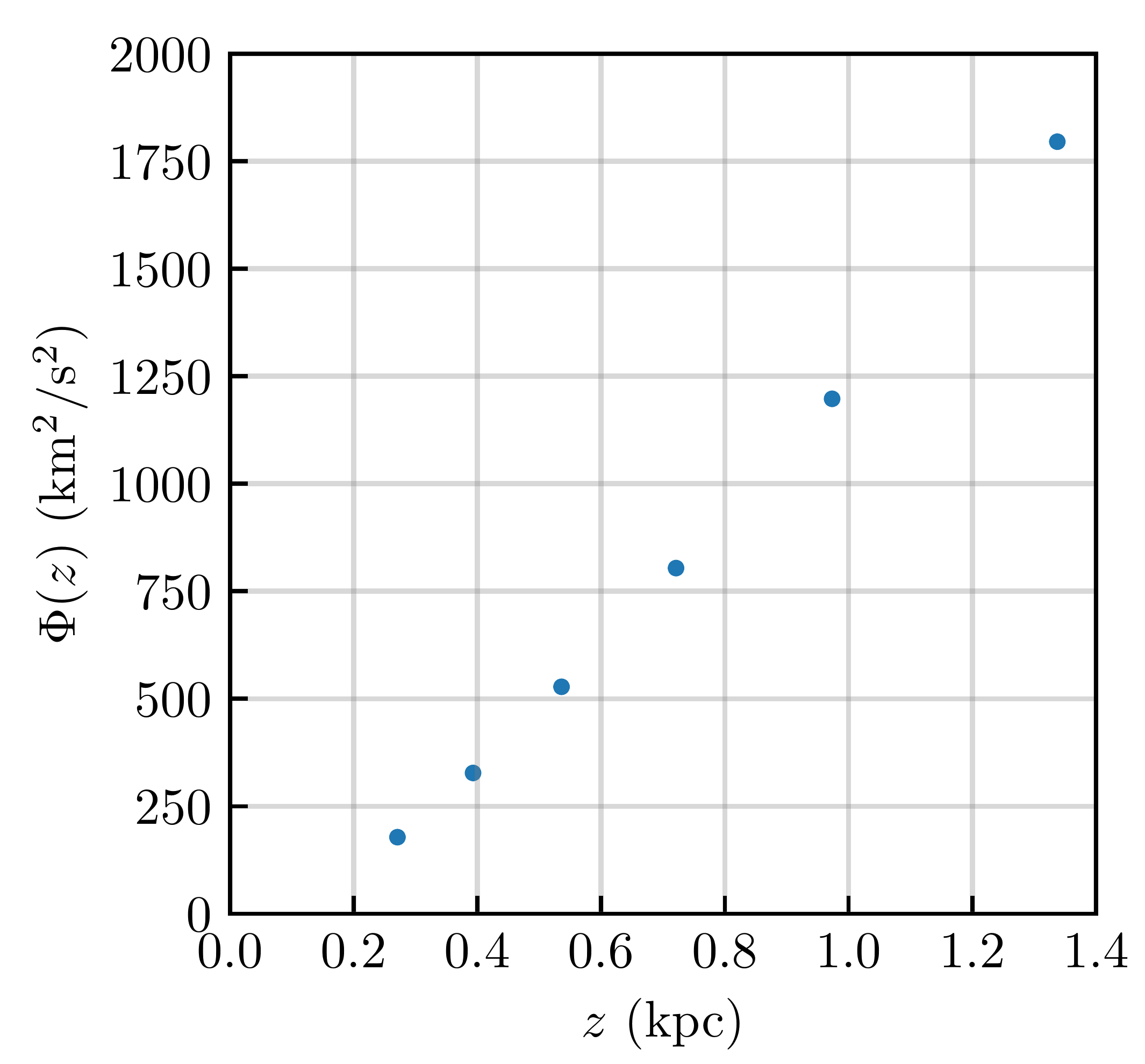
If we follow the trajectory of a single star that lies on the spiral, we would find it oscillating around the mid-plane with some period $T(z)$ that decreases with increasing $z$. Over the course of an orbit, the energy per unit mass is conserved and is given by $E = v_z^2/2 + \Phi(z)$. We know that near the mid-plane, the gravitational potential is minimal and equal to zero, so $v_z$ is maximal and the kinetic energy equals the total energy. Hence, we know the total energy of stars at the seven intersection points of the spiral with $z = 0$. Similarly, when $v_z = 0$, the kinetic energy is zero, so the total energy equals $\Phi(z)$ at those points.

As one traces the various intersection points with $v_z = 0$ and $z = 0$ along the spiral, the maximal extent of the orbit keeps increasing. To the first order, assuming the maximal extent increases linearly with each crossing, we can find the potential energy of the crossings of $v_z = 0$ as the average between the kinetic energies of the previous and subsequent crossing over $z = 0$. This allows us to determine the potential energy at all the crossings with $v_z = 0$, as tabulated below.

$i$	$z_i$ (kpc)	$\Phi(z_i)$ (km²/s²)
1	0.27	180
2	0.39	330
3	0.54	530
4	0.72	800
5	0.97	1200
6	1.34	1800

Grading (preliminary)

• Making use of the total energy at $z = 0$ intersection points being known (either explicitly or implicitly): 0.7 pts
• Interpolating the values at $v_z = 0$ from neighbouring $z = 0$ crossovers (should be explicitly mentioned): 0.8 pts
• Tabulating the potential:
  • Using six points: 0.7 pts
  • Using four to five points: 0.4 pts
  • Using one to three points: 0.1 pts
• $\Phi(z)$ vs $z$ correctly plotted: 0.3 pts

---

Part iv (1 point)

For a harmonic oscillator, the potential energy would grow as $z^2$. Based on the plot of potential energy we obtained, it seems to grow roughly quadratically in the beginning, and then transition into a more linear regime, implying that smaller values of $z$ have more uniform $\rho$. Taking the first value of $\Phi(z_1) = 180\,\text{km}^2\text{s}^{-2}$ and using $\Phi(z) = \int a_z\,dz = 2\pi G\rho_0 z^2$:

$$\rho_0 = \frac{\Phi(z_1)}{2\pi G z_1^2} = 6.1\times 10^{-21}\,\text{kg\,m}^{-3} = 0.090\,M_\odot\text{pc}^{-3}.$$

Grading (preliminary)

• Connecting $\Phi(z_1)$ with $\rho_0$ by assuming constant mass density: 0.8 pts
• If the first data point is not used: −0.2 pts
• Final expression for $\rho_0$: 0.1 pts
• Numerical value within 10%: 0.1 pts

---

Part v (2 points)

We can compute the enclosed surface density $\Sigma(z)$ between $0 < z$ by using the previous harmonic oscillator estimate. With the constant density approximation:

$$\Sigma(z) = \rho_0 z = \frac{\Phi(z)}{2\pi G z}.$$

(Here $\rho_0$ is a placeholder variable while using the constant profile approximation to simplify the calculus. The final result is expected to deviate from the true value by a numerical factor close to unity.)

Assuming dark matter density dominates far away, we can use the difference between the farthest two data points at $z_5$ and $z_6$ to estimate the dark matter density:

$$\Sigma(z_6) - \Sigma(z_5) = \rho_\text{DM}(z_6 - z_5) = \frac{1}{2\pi G}\left(\frac{\Phi(z_6)}{z_6} - \frac{\Phi(z_5)}{z_5}\right).$$

Thus,

$$\rho_\text{DM} \approx \frac{1}{2\pi G(z_6 - z_5)}\left(\frac{\Phi(z_6)}{z_6} - \frac{\Phi(z_5)}{z_5}\right) = 7.7\times 10^{-22}\,\text{kg\,m}^{-3} = 0.011\,M_\odot\text{pc}^{-3}.$$

Dark matter therefore makes up around $\rho_\text{DM}/\rho_0 = 13\%$ of the total local matter budget.

Grading (preliminary)

• Obtaining an expression for the total mass contained within $z$: 0.7 pts
• Taking the difference between the total mass within $z_6$ and $z_5$ for calculating the dark matter content: 0.9 pts
• Final expression for $\rho_\text{DM}$ based on $z_6$ and $z_5$: 0.3 pts
• Numerical value within 10%: 0.1 pts

Alternative scheme:

• Using the previous expression for $\rho$ based on $\Phi(z)$ to express $(z_6 - z_5)\rho_\text{DM} = z_6\rho(z_6) - z_5\rho(z_5)$: 1.6 pts
• Final expression for $\rho_\text{DM}$ based on $z_6$ and $z_5$: 0.3 pts
• Numerical value within 10%: 0.1 pts

---

Part vi (2 points)

We can estimate the time of the perturbation by using the winding rate between two points on the spiral and how many full turns around the origin they have made relative to each other. Using the harmonic estimate, $\rho_0 = \Phi(z)/(2\pi Gz^2)$ and the angular frequency is

$$\omega(z) = \sqrt{4\pi G\rho_0} = \sqrt{2\Phi(z)/z^2}.$$

Picking points $z_1$ and $z_6$ and seeing that they have 2.5 full turns between them, we can express how long ago the perturbation happened:

$$T_0 = 2.5\cdot\frac{2\pi}{\omega(z_1) - \omega(z_6)} = 5\pi\left(\sqrt{\frac{2\Phi(z_1)}{z_1^2}} - \sqrt{\frac{2\Phi(z_6)}{z_6^2}}\right)^{-1}$$ $$= 1.9\times 10^{16}\,\text{s} = 620\,\text{Myr}.$$

The timescale is relatively long, but compared to the lifespan of the Milky Way, which is around 13.6 billion years, it’s relatively recent.

Grading (preliminary)

• Idea of using differences in the winding rate between two points on the spiral: 1.0 pts
• Expression for angular frequency $\omega$ in terms of $\Phi(z)$ by assuming a harmonic oscillator: 0.5 pts
• Picking two points and connecting the age of the spiral, $\omega$ and the winding amount: 0.3 pts
• Numerical value within 10% of the solution value: 0.2 pts